


Manually copying and pasting values from one sheet to another is such a time-wasting process. Not to mention, each time you add a new value in “Sheet A”, it won’t magically appear in “Sheet B”, and vice versa.
The better option would be to link those two spreadsheets using Excel formulas, which I’ll explain in this tutorial.
How to pull data from another sheet in Excel
To pull data from one spreadsheet to another, it's actually pretty simple. Just specify the cell being copied into the destination cell.
For instance, you've got a value in cell C8 of Sheet1. And you want the data to appear in cell B6 of Sheet2. To sync the value, open cell B6 of Sheet2 and enter this formula:
=Sheet1!C8

But there are also other Excel functions you can use to pull data from a worksheet to another, including INDEX and VLOOKUP.
How to pull data from another Excel sheet using the INDEX function
INDEX is an Excel command to scan an array or data range inside a sheet, and pull data from specific "coordinates" (row number and column number) within that area.
=INDEX(array;row_num;column_num)
So if you want the value inside cell B5 of Sheet1 to appear in another sheet.
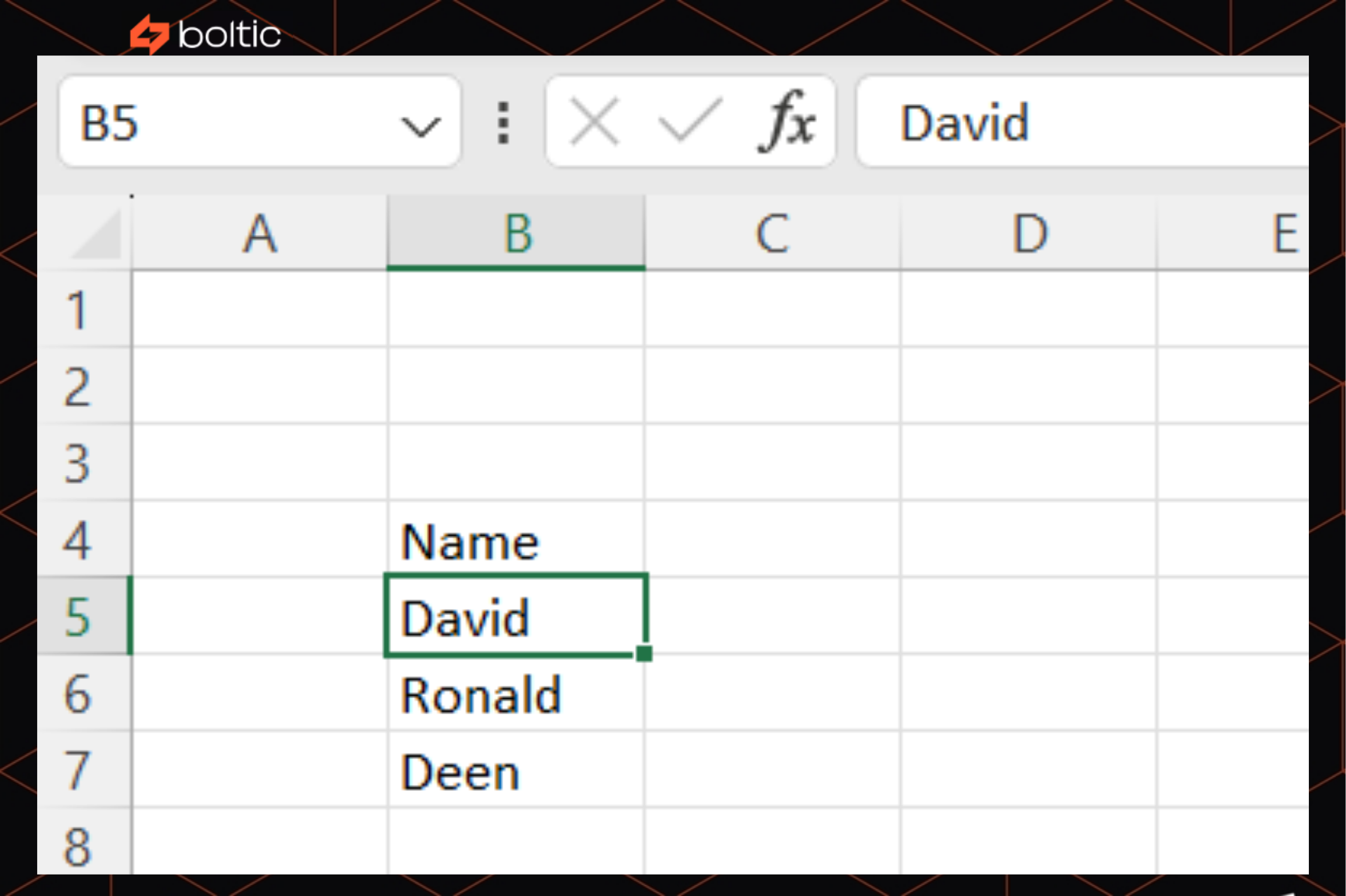
Open your destination cell and enter:
=INDEX(Sheet1!A1:D13;5;2)
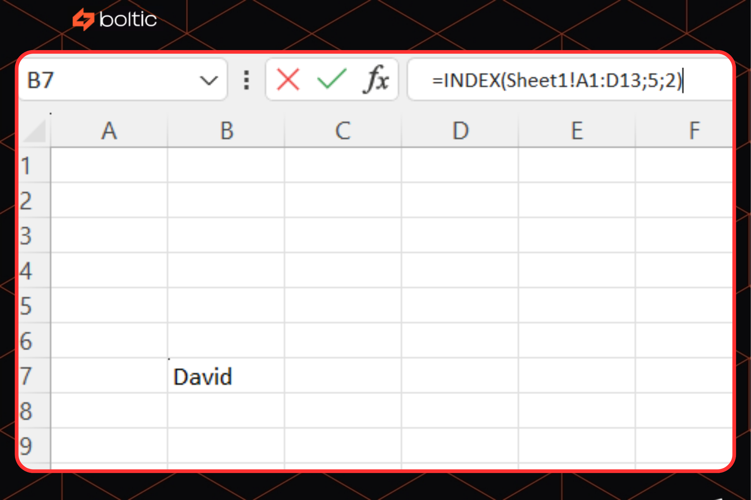
Explanation:
- Sheet1!A1:D13 – is your array. It tells Excel to look within the range A1 to D13 on "Sheet1".
- 5 – is the row_num. It tells Excel to pull data from row 5 within that array.
- 2 – is the column_num. It tells Excel to pull data from the 2nd column (or column B) within that array.
How to pull data from another Excel sheet using the VLOOKUP function
VLOOKUP is widely used to find specific values in a table or data range, and then retrieve those to different columns in another sheet.
=VLOOKUP(lookup_value;table_array;col_index_num;[range_lookup])
- lookup_value – the exact reference point. This could be a cell (A2), or a hardcoded value ("Product A").
- table_array – the range of cells where Excel will look for your lookup_value and from which it will retrieve the matching data.
- col_index_num – the column number within the table_array that contains the value you want to return. The leftmost column in your table_array is always column 1.
- [range_lookup] – an optional argument for getting an exact match or an approximate match value. TRUE or omitted: Approximate match. The table_array's first column must be sorted in ascending order. FALSE: Exact match. This is what you'll use almost always for precise lookups.
Sounds confusing? I’ll show you how it works.
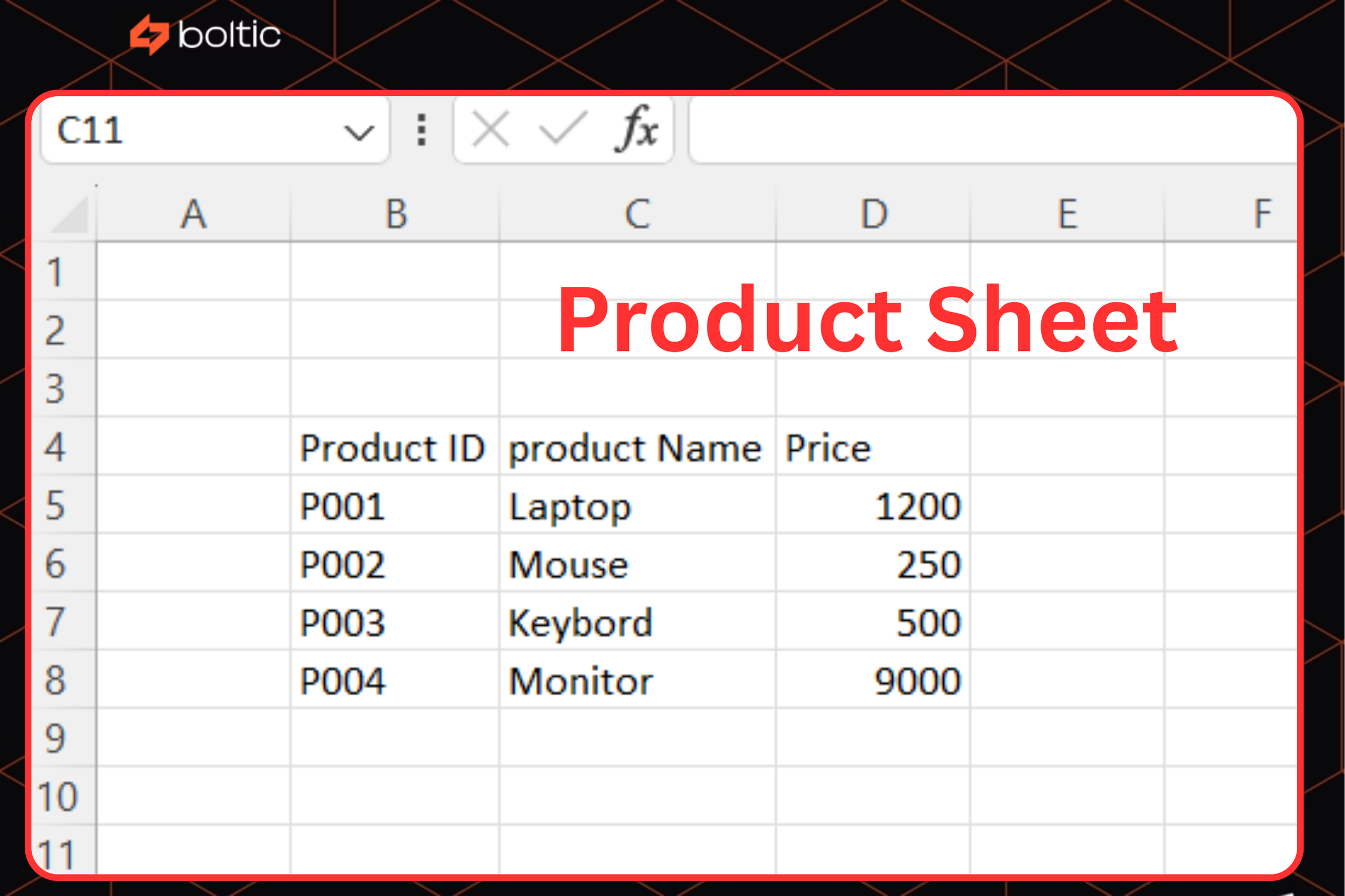
You have two spreadsheets in the same Excel workbook. The first one contains product information you want to pull. Let’s call it a “Product” sheet.
While the second one is a “Report” worksheet where you want to display the retrieved product data.
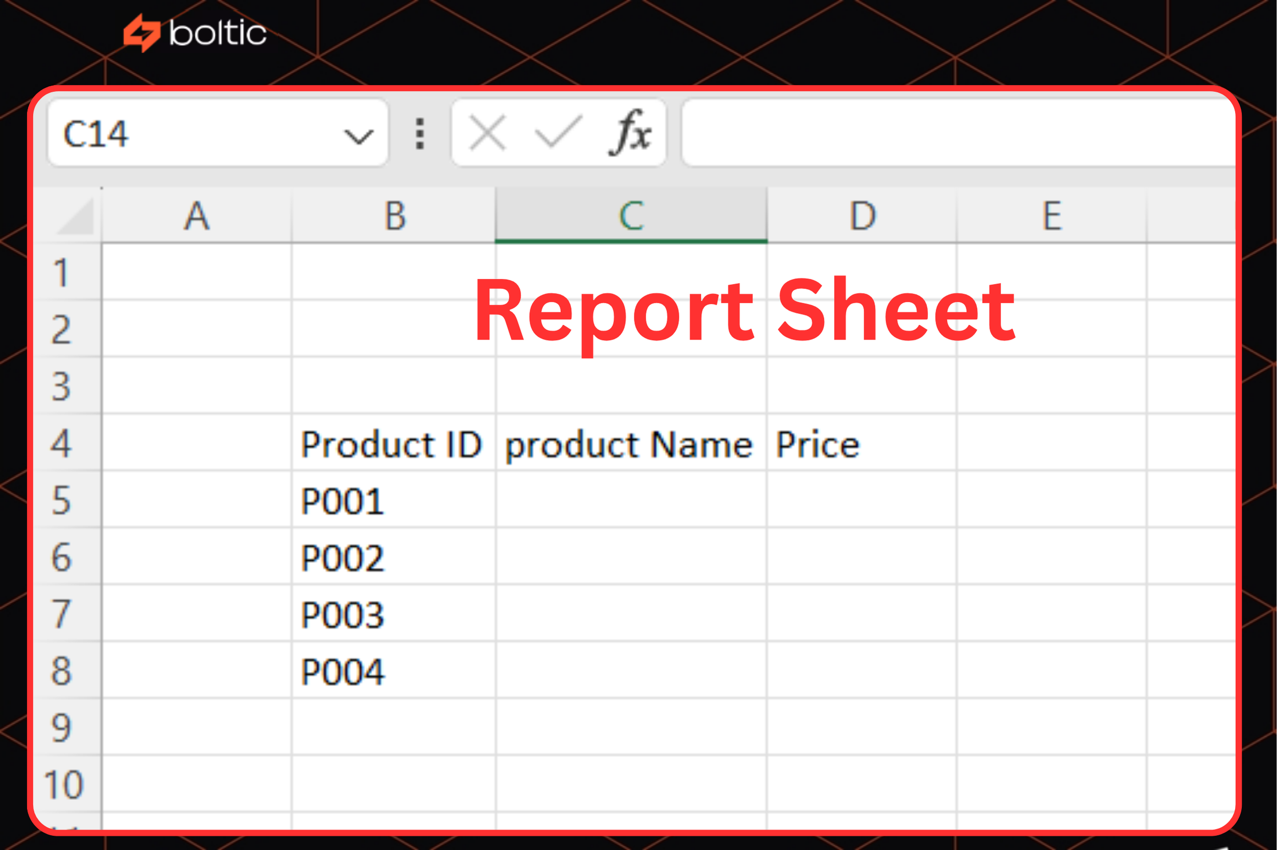
Now, your goal is to populate the “Product Name” column in the “Report” sheet. To do that, you'll have to retrieve the value from the relevant cell in the “Product” sheet:
Step 1 - Go to the “Report” sheet.
Step 2 - Select the cell where you want the product name to appear. Since you want to populate the first product name column, it should be C5.
Step 3 - Input this to that cell: =VLOOKUP(B5, Product!B5:C100, 5, FALSE).
Step 4 - Press Enter. Excel will look up a product ID in B5 and return the product name from the fifth column of the Product sheet.
Step 5 - Cell C5 should now show "Laptop". Drag the fill handle (the small square at the bottom-right of cell C5) down to C7 to apply the formula to "Mouse" and "Keyboard".
How to aggregate data from multiple Excel Sheets
Below, you'll find the steps to combine and sum up data from multiple sheets and workbooks with the Consolidate command, Power Query function, and SUMIFS formula.
How to aggregate data from multiple Excel sheets using the Consolidate tool
Looking to calculate the value of multiple datasets from different sheets? You can use the data consolidation feature:
Step 1 - Open the sheet where you want to add the consolidated data to.
Step 2 - Head to Data → Consolidate.
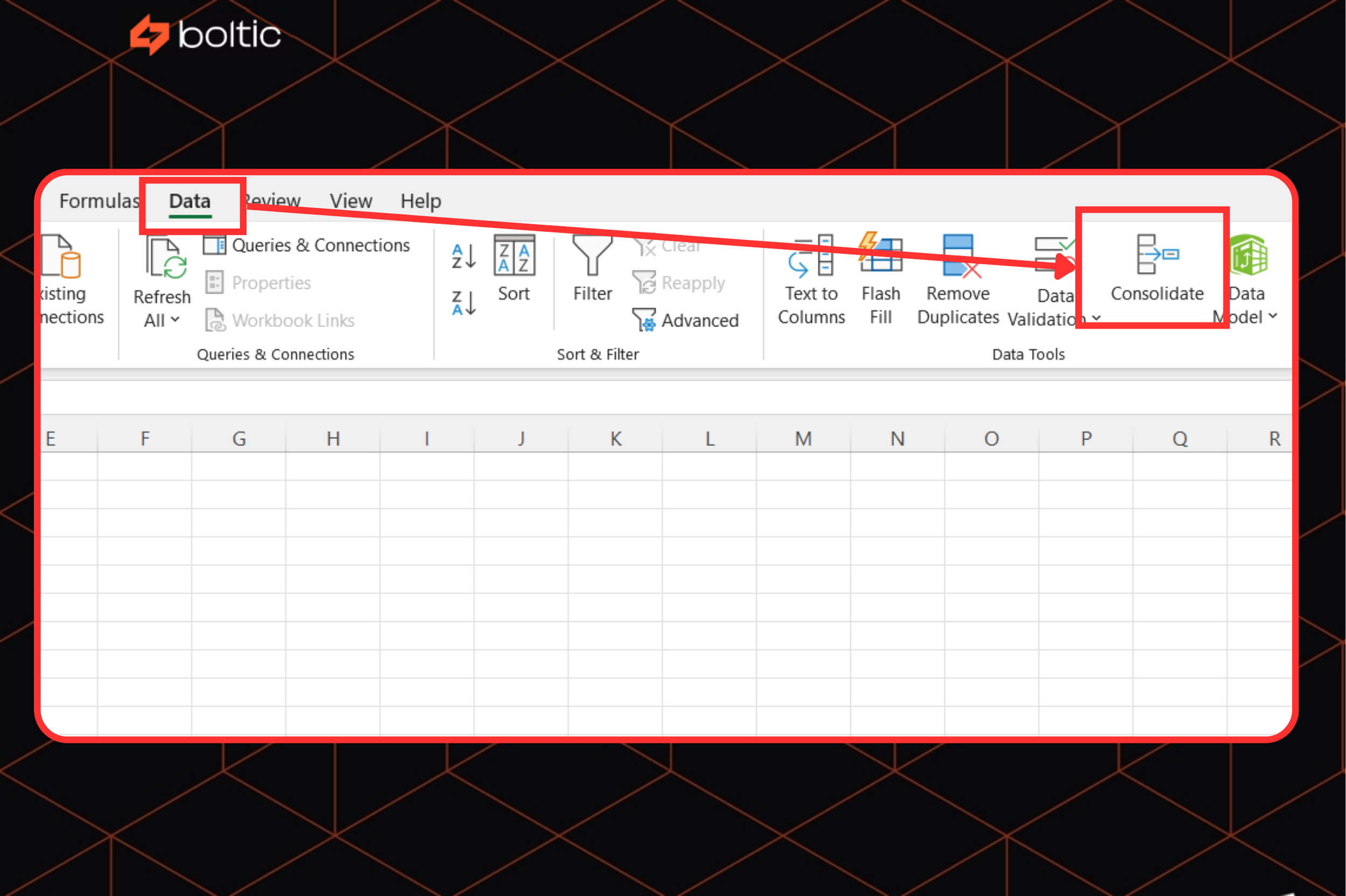
Step 3 - From the Consolidate window that appears, select the function you want to use from the dropdown.
Step 4 - Click the Reference field, then go to your first sheet and select the range you want to pull in. Click the + button to include it.
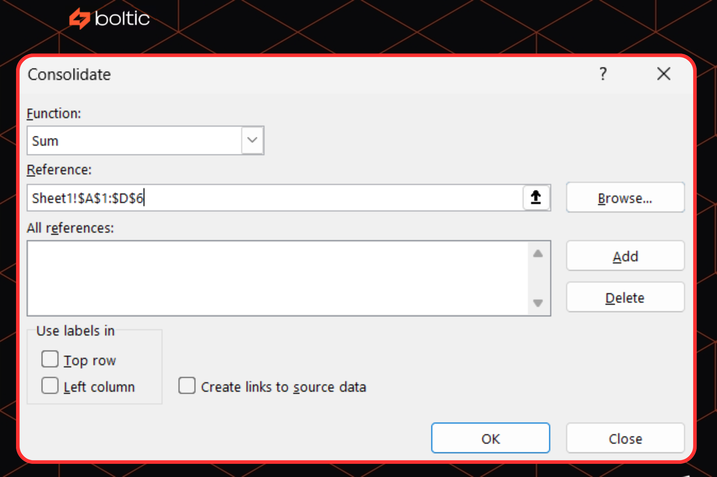
Step 5 - Repeat for each additional sheet or workbook.
Step 6 - Once you’ve added all your data ranges, click OK.
How to aggregate data from multiple Excel sheets using the Power Query feature
Power Query is a tool for combining data from multiple sheets into a single dataset.
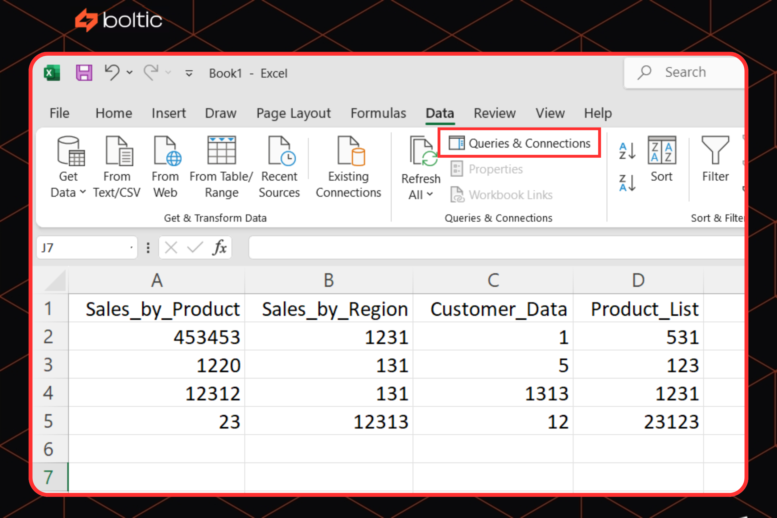
Imagine this. You have an Excel workbook file, let's just call it SalesReport2025.xlsx. It contains various sheets:
- Sales_by_Product
- Sales_by_Region
- Customer_Data
- Product_List
And now, your goal is to merge the Sales_by_Product and Sales_by_Region sheets.
To do that:
Step 1 - Create a new Excel workbook for the new combined data.
Step 2 - Click Data → Get Data (Power Query) from the top menu.
Step 3 - You’ll be asked to choose a data source. Select Excel workbook.
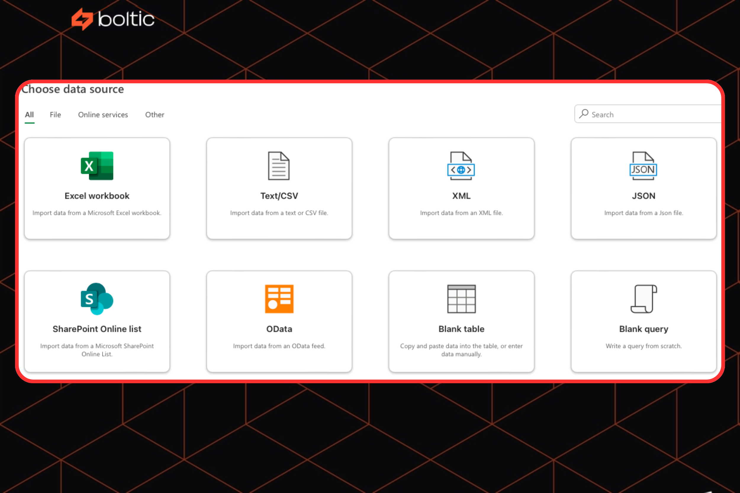
Step 4 - Click Browse and select the workbook you want to query.
Step 5 - Click Import and the Navigator window will appear. It shows you all the sheets and Excel Tables found within the selected workbook.
Step 6 - Check the box that says Select multiple items. Then select each sheet you want to retrieve and combine data from.
Step 7 - Click Transform Data.
The Power Query Editor would appear. From there, you'll see a separate query for each sheet you've selected before.
To combine those sheets:
Step 1 - Select one of your sales queries in the Queries pane on the left.
Step 2 - Open the Home tab, then click Append Queries (dropdown arrow) → Append Queries as New.
Step 3 - In the Append dialog box, select Three or more tables.
Step 4 - Add all your relevant sales queries to the Tables to append list.
Step 5 - Click OK.
A new query (often named Append1) will be created.
Finally, open the Home tab and click Close & Load. Your combined data from multiple sheets will now appear as a single, clean Excel Table.
Dynamic data retrieval using the INDIRECT function
Use INDIRECT to turn text values into actual cell or range references. This allows your formulas to respond to changes in sheet names, cell addresses, or user input — without having to rewrite the formula each time.
Say your sheet has:
- Cell A1 has value "10"
- Cell B1 has value "A1"
Now, if you write =B1 in another cell, Excel just gives you whatever is literally in B1 – which would be the text "A1".
But if you write =INDIRECT(B1), something different happens. Excel reads what's in B1 (the text "A1"), then uses that text as directions to go find cell A1, and brings back the value from there – which is 10.h
Note: INDIRECT() does not work with closed workbooks. The referenced sheet must be open in Excel.
How to automate the process of pulling spreadsheet data
Is there a way to automate data pulling and management in Excel? Yes, with VBA (Visual Basic for Applications).
Use VBA when:
- You regularly pull the same type of data from multiple sheets or workbooks.
- You want to reduce manual work.
- You need more flexibility than Excel formulas allow
To access the VBA editor, follow the steps laid out on Microsoft’s help page.
Here are some basic VBA scripts you can use:
Pulling data from another sheet in the same workbook
Pulling data from a closed workbook (most common for automation)
Common issues when pulling information from another Excel worksheet
Below are some issues that often happen when you pull data from an Excel sheet and how to fix them.
#REF! error
This error occurs when a reference is invalid. Usually because a cell, column, or sheet was deleted, or exists outside a valid range.
For example, VLOOKUP(A1, B1:C10, 3, FALSE) would result in a #REF! error. Why? Because B1:C10 only has two columns, but you're asking for the 3rd.
If you see this error, keep calm. Click on the cell that’s showing #REF! and look at the formula bar to identify the parts of the formula that are causing the error.
Check whether the sheet, cell, or data range it references is still there. Also, make sure you are not requesting a column number or index that is out of range like the example above.
If the reference sheet, cell, or data range is missing, re-select the correct one. You can also use named ranges or Excel Tables to avoid hard-coded references, which I’ll explain later.
Circular reference warning
A circular reference usually happens when a formula refers to its own cell, whether directly or indirectly. As such, this creates an infinite loop.
For instance, if you type =A1+5 into cell A1, you've created a direct circular reference. Excel needs to know the value of A1 to calculate A1+5, but A1's value is A1+5. So it's a never-ending loop.
Another example:
- In cell A1, you type =B1+10.
- In cell B1, you type =A1*2.
Here, A1 depends on B1, and B1 depends on A1, forming a loop. Excel won't be able to determine a final value for either.
To fix this, go to the Formulas tab → Error Checking → Circular References. This menu will list all cells involved in circular references. Clicking on a cell in this list will take you directly to it.
Once you've identified a cell involved, click Trace Precedents from the main Formulas tab to see cells that affect the current cell and Trace Dependents to see cells that are affected by the current cell. By doing so, you can visually map out the formula dependencies and identify the loop.
Best practices for organizing data in Excel
In Excel, even the smallest mistake can lead to data retrieval errors. Maybe you've added an extra space to your formula. Maybe there's a missing value or inconsistent formatting.
Thus, if you want to ensure accuracy, maintain data integrity, and make your spreadsheets easier to manage and scale, follow these best practices:
Structure your data as a table
An Excel Table makes your data easier to analyze, reference, and format. Each time you add new values, it automatically expands to include new rows or columns. As such, your formulas will always reference the latest and correct dataset, greatly minimizing errors.
Simply select a cell range containing your data. Then, press Ctrl + T to transform those rows and columns into an Excel Table.
Simplify Excel formulas with named ranges
Want your formulas to be easier to read and less prone to errors? Named ranges are a great solution.
Instead of a cryptic cell reference like Sheet1!$D$2:$D$500, a named range makes it possible to assign a descriptive name to a cell or range, such as Sales_Jan or Client_New.
This undoubtedly brings nice advantages:
- Readability: =SUM(Total_Sales_Amount) is easier to understand, memorize, and execute than =SUM(Sheet1!$D$2:$D$500)).
- Robustness: If you add or delete rows/columns within a named range, the range automatically adjusts. So, your formulas will always reference the correct cells. However, static named ranges only adjust for inserted/deleted rows inside the range but won’t expand automatically. Use Excel Tables (Ctrl + T) for that.
- Easy finding: You can easily find any named range by typing it in the Name Box (located left of the formula bar).
Here’s how you give your cells a name:
Step 1 - Select the cell range you wish to name.
Step 2 - Click the Name Box (located in the left of the formula bar).
Step 3 - Type your desired name. Remember these rules: No spaces. Use underscores (_) or periods (.) instead like Sales_March, Customer_ID, or Best.Seller. The name can’t start with a number, can’t be the same as a cell reference (e.g., A1), and it can only be 255 characters long.
Step 4 - Press Enter.
drives valuable insights
Organize your big data operations with a free forever plan
An agentic platform revolutionizing workflow management and automation through AI-driven solutions. It enables seamless tool integration, real-time decision-making, and enhanced productivity
Here’s what we do in the meeting:
- Experience Fynd Boltic's features firsthand.
- Learn how to automate your data workflows.
- Get answers to your specific questions.