

When you manage a large amount of data, mistakes happen. Maybe somebody in your team inputs the same data you’ve already entered earlier in the morning. Or maybe you paste the same text twice in different rows.
Luckily, whatever the reason, spotting and deleting duplicate data in Google Sheets are pretty easy. In this article, I’ll show you how to find and remove duplicates using Google Sheets’ native tools and extensions.
How to find duplicates in Google Sheets
Google Sheets has native functions that allow you to scan for duplicate records: Conditional Formatting and Pivot Tables. In this section, I'll walk you through the steps to use them.
How to find duplicate values using Conditional Formatting
Here’s how to highlight the exact same values within a single column:
Step 1 - Select the data range that you want to check for duplicate information.

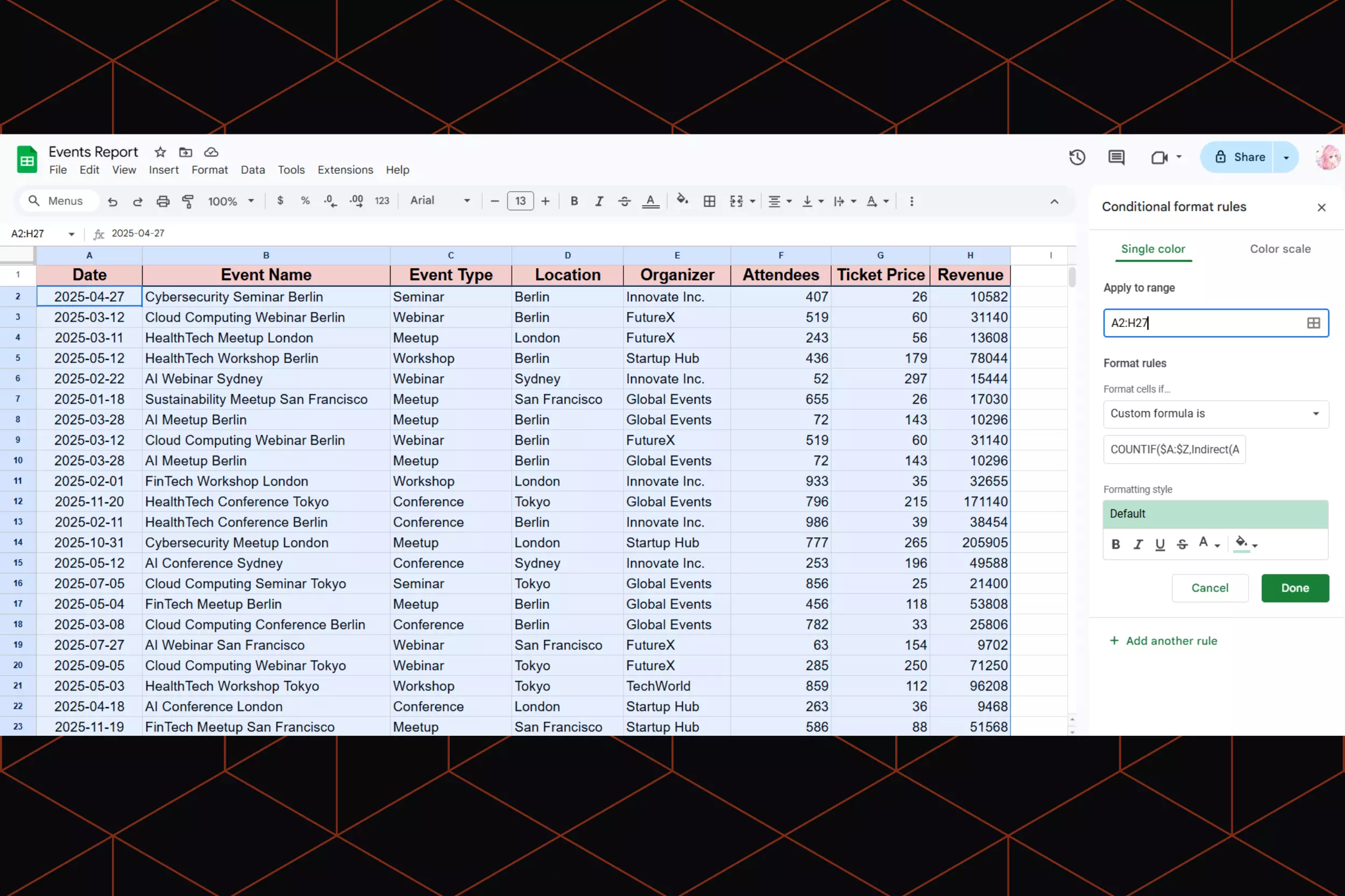
Step 2 - From the top menu bar, head over to Format → Conditional Formatting.

Step 3 - The Conditional format rules window will appear on the right side of your screen. From there, click the dropdown menu under Format rules and choose the Custom formula is option.
Step 4 - Enter the COUNTIF formula in the “Value or formula” field based on your chosen data range. Since I've selected cells A3:A25 before, the custom formula will be =COUNTIF($A$3:$A$25,A3)>1.
.gif)
Step 5 - By default, your duplicate records will be highlighted in green. But you can change the highlight color under Formatting style.
.gif)
Keep in mind that conditional formatting will only highlight duplicates, not delete them. So after following the steps above, you can then delete each duplicate row yourself. If you want to spot duplicate records in multiple rows and columns, it's also possible. Simply select all applicable cells and use this formula:
=COUNTIF($A:$Z,Indirect(Address(Row(),Column(),)))>1
You can also change the Apply to range field to check for duplicates in specific rows and columns. All duplicate values within selected cells will be highlighted in green.
How to find duplicate values using Pivot Table
Pivot Table is another tool you can use to find out whether certain values have duplicates, and how many.
Here’s how to create a Pivot Table:
Step 1 - Select all cells containing the data you want to check for duplicates. Then, Head over to the top menu and go to Insert → Pivot table.
.gif)
Step 2 - You can either insert the Pivot Table in the existing sheet or a new one. I recommend going with a new sheet for more clarity.
.gif)
Step 3 - From the Pivot table editor, select the column name you want to check for duplicates under Rows.
Step 4 - Then, scroll down to Values → Summarize by and choose COUNTA from the dropdown menu.

Step 5 - The Pivot Table will then show you the count for each value – duplicate values will have a count greater than 1.
.gif)
How to remove duplicates in Google Sheets
If you prefer to delete duplicate data straight away without reviewing it first, you can use the native data cleanup tool in Google Sheets.
How to remove duplicates using the Data Cleanup tool
Here's how to automatically delete all duplicate values in Google Sheets:
Precaution: the following method will delete all your duplicate data permanently. So, I recommend making a copy of your sheet before you proceed.
Step 1 - Highlight the specific data you want to check for duplicates. Or, if you want to scan all cells, click the top left corner of your sheet.

Step 2 - From the top toolbar, head to Data → Data cleanup → Remove duplicates.
.gif)
Step 3 - Once the Remove duplicates box appears, select all the columns you want to check for duplicate information. If you have a header row, also make sure to tick the Data has header row box, so Google Sheets won’t remove any duplicate title.
.gif)
Step 4 - Click Remove duplicates, and all your duplicate records will be deleted. If the process is successful, you’ll see a report on the number of duplicate rows removed, and how many unique rows remain.

How to remove duplicates using Apps Script
If you don’t want to repeat the steps I’ve mentioned above each time you want to remove duplicates, you can automate the process with Apps Script.
You just need to set it up once, and then simply run the script over and over again when you add new data:
Step 1 - Open the sheet where you want to remove duplicates.
Step 2 - From the top menu, head to Extensions → Apps Script.
.gif)
Step 3 - In the Apps Script editor, enter this script to the Code.gs file:
/**
 * Removes duplicate rows from the active Google Sheet,
 * keeping only the first occurrence of each unique row.
 * A custom menu item will be added to easily run this function.
 */
function onOpen() {
  SpreadsheetApp.getUi()
      .createMenu('Deduplicate')
      .addItem('Remove All Duplicates (Keep First)', 'removeDuplicates')
      .addToUi();
}

function removeDuplicates() {
  const sheet = SpreadsheetApp.getActiveSpreadsheet().getActiveSheet();
  const range = sheet.getDataRange(); // Gets all data with content
  const values = range.getValues();   // Gets the values as a 2D array

  const uniqueValues = [];
  const seenRows = new Set(); // Stores stringified versions of rows

  for (let i = 0; i < values.length; i++) {
    const row = values[i];
    const rowString = JSON.stringify(row); // Convert row to a unique string for Set lookup

    if (!seenRows.has(rowString)) {
      uniqueValues.push(row);
      seenRows.add(rowString);
    }
  }

  // Clear existing data and write back only the unique rows
  sheet.clearContents();
  if (uniqueValues.length > 0) {
    sheet.getRange(1, 1, uniqueValues.length, uniqueValues[0].length).setValues(uniqueValues);
  }

  SpreadsheetApp.getUi().alert('Success!', 'All duplicate rows removed, keeping the first occurrence.', SpreadsheetApp.getUi().ButtonSet.OK);
}
Step 4 - Give your project a name (like “delete duplicates”) and click Save project to Drive to save your script.
.gif)
Step 5 - Go back to your sheet and reload the page. You’ll now see a new menu called Deduplicate.
Step 6 - Click Deduplicate → Remove All Duplicates (Keep First).

Step 7 - Give the Apps Script permission to access your Google Sheet.
Note: Google displays a security warning for unverified scripts. If you see this, just click Advanced, then Go to [Project Name] (unsafe) to proceed.
Step 8. Run your deduplicate script. If the process is successful, you’ll see the message below.

How to remove duplicates using a Google Sheets add-on
Don't want to deal with complex formulas or scripts? The Remove Duplicates extension makes the process a lot easier.
Here’s how it works:
Step 1 - Install Remove Duplicates.
Step 2 - Open your sheet and head to Extensions → Remove Duplicates → Find duplicate or unique rows.
.gif)
Step 3 - A new window will pop up. From there, select your cell range and choose to find Duplicates.
Step 4 - Decide what you want to do with the duplicate cells: you can either highlight them with a certain color, move them to another location, or simply clear the values within the duplicate rows.

Step 5 - Click Finish to proceed with your desired action.
Bonus Google Sheets tutorials
How to extract unique values in Google Sheets
If you want to extract unique values (non-duplicated entries) while keeping your original data, you can use the UNIQUE function:
Step 1 - Select an empty cell in your sheet.
Step 2 - Go to the formula bar.
Step 3 - Enter the =UNIQUE function based on your cell range. For example: =UNIQUE(A5:B14).

How to split data into columns
Copying and pasting your text to different columns manually is time-consuming. The good news is, Google Sheets’ text splitting function allows you to split a cell that, for example, contains “Name, Email,” into two columns: "Name" and "Email."
Here's how:
Step 1 - Type your text, or paste it into your sheet.
Step 2 - From the top toolbar, click Data → Split text to columns.

Step 3 - Open the Separator dropdown menu and select the character you used to separate your text.

How to remove extra spaces
To remove extra spaces in your sheet, select the cell range you want to clean. Then, click Data → Data cleanup → Trim whitespace.
.gif)
Note: you can’t use this method to remove empty cells and non-breaking spaces (like  ).
How to connect Google Sheets with other apps you use
Boltic gives you the power to integrate Google Sheets with other software, tools, and apps in your system, so you can sync your data and automate your business processes.
You can run workflows that automatically read, write, or update data in your Google Sheet files. For example, when your sales representative updates a customer record in your CRM (like Salesforce or HubSpot), our system will automatically update the corresponding row in your sheet.
Sounds tempting? Visit our documentation page for more information on how to set up a Google Sheets integration in Boltic.
drives valuable insights
Organize your big data operations with a free forever plan
An agentic platform revolutionizing workflow management and automation through AI-driven solutions. It enables seamless tool integration, real-time decision-making, and enhanced productivity
Here’s what we do in the meeting:
- Experience Boltic's features firsthand.
- Learn how to automate your data workflows.
- Get answers to your specific questions.

